Key summary
Backpropagation is the method of passing the difference between a neural network’s output and the target (the loss) backward from the output layer toward the input layer, using the chain rule to calculate how much each weight is responsible for the loss (its gradient). Moving each weight slightly in the direction opposite to that gradient is gradient descent, and repeating the two steps is how a network learns.
Backpropagation is the core procedure a multi-layer neural network uses to figure out which direction and how much to adjust each weight when its prediction differs from the target. This post walks through the four-step training loop, what a gradient tells us, a hand-checked chain rule example, and how backpropagation differs from gradient descent.
What is backpropagation?
One-line answer: It is the procedure that passes the loss between the forward-pass output and the target backward from the output side toward the input side to compute each weight’s gradient.
One training step in a neural network repeats the following four stages:
- Forward pass: feed the input through the network to compute the output.
- Loss computation: measure the difference between the network’s output and the desired target.
- Backward pass (Backpropagation): compute each weight’s gradient with the chain rule, working backward from the output side toward the input side.
- Weight update: move each weight a little in the direction opposite to its gradient (gradient descent), and repeat the loop.
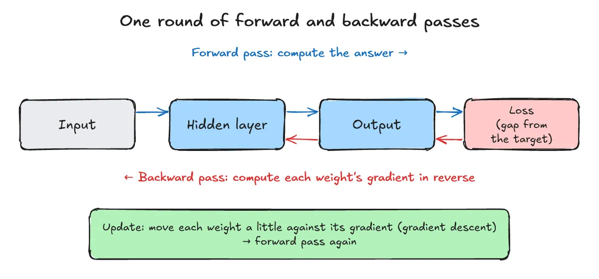
Rumelhart, Hinton & Williams (Learning representations by back-propagating errors, Nature 323, 533–536, published 9 October 1986) is the well-known paper that described and popularized this procedure for multi-layer networks. It describes back-propagation as a learning procedure for networks of neurone-like units that repeatedly adjusts connection weights to minimize a measure of the difference between the network’s actual output vector and the desired output vector; as a result, internal hidden units come to represent important features of the task.
How training stages such as pre-training and fine-tuning are distinguished is covered in Pre-training, fine-tuning, and RLHF differences: What stages build an LLM?.
What does a gradient tell us?
One-line answer: Its sign tells whether increasing a weight slightly makes the loss go up or down, and its size tells how sensitive the loss is to that change.
The gradient computed for each weight carries two pieces of information:
- Sign: tells whether increasing the weight a little increases or decreases the loss.
- Size: tells how sensitive the loss is to changes in that weight.
You can think of it like standing on a mountain in thick fog: even when you cannot see the valley, you can feel the slope under your feet and step downhill in the direction opposite to the upward slope.
How is the chain rule used in backpropagation?
One-line answer: It multiplies the gradient arriving from the output side by each operation node’s local gradient step by step to find the gradients of earlier weights.
Consider a small computation graph with a multiplication node u = w * x, an addition node z = u + b, and a loss L = (z - t)^2, where x = 2, w = 3, b = 1, and the target t = 5.
u = w * x
z = u + b
L = (z - t)^2

x = 2, w = 3, b = 1, t = 5
Forward:  u = 3 * 2 = 6,  z = 6 + 1 = 7,  L = (7 - 5)^2 = 4
Backward: dL/dz = 2 * (z - t) = 2 * 2 = 4
          dL/du = 4,  dL/db = 4
          dL/dw = dL/du * x = 4 * 2 = 8
          dL/dx = dL/du * w = 4 * 3 = 12
Walking through the forward and backward passes step by step:
- Forward pass:
u = 3 * 2 = 6,z = 6 + 1 = 7, and the loss isL = (7 - 5)^2 = 4. - Gradient of the loss with respect to the output:
dL/dz = 2 * (z - t) = 2 * 2 = 4. - Addition node (
z = u + b) backward: an add node passes the incoming gradient unchanged to both of its inputs, sodL/du = 4anddL/db = 4. - Multiplication node (
u = w * x) backward: a multiply node multiplies the incoming gradient by the other input, givingdL/dw = dL/du * x = 4 * 2 = 8anddL/dx = dL/du * w = 4 * 3 = 12.
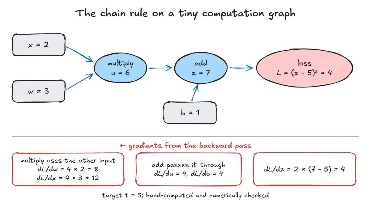
Because dL/dw = 8 is positive, increasing w a little increases the loss, so gradient descent decreases w.
How does backpropagation differ from gradient descent?
One-line answer: Backpropagation is the step that computes the gradient for each weight, whereas gradient descent is the step that uses those gradients to update the weights.
Although the two terms are often mentioned together, they refer to distinct parts of the training loop:
- Backpropagation: computing each weight’s gradient with the chain rule from the output side back toward the input side.
- Gradient descent: using those computed gradients to move each weight slightly in the opposite direction to reduce the loss.
How far to move on each step is covered in a separate post, “What is a learning rate?”.
What are the frequently asked questions?
One-line answer: Here are answers to three common questions covering vanishing gradients, automatic differentiation, and whether backpropagation runs during inference.
What is the vanishing gradient problem?
In deep networks, multiplying many small local gradients along the chain can make gradients near the input side very small, so those weights barely change. Activation function choice is one factor, which is covered in a separate post, “What is an activation function?”.
Do frameworks run backpropagation automatically?
Yes. Deep learning frameworks compute the gradient of each weight automatically through automatic differentiation.
Does backpropagation run during inference?
No. Inference with a trained model runs only the forward pass; there is no backpropagation and no weight update.
What related posts are worth reading?
One-line answer: You can check our related posts on language model training stages, overfitting, and AI basics study notes.
- Pre-training, fine-tuning, and RLHF differences: What stages build an LLM?
- What is overfitting?
- AI basics study notes (Korean)
What are the sources?
One-line answer: This post references the 1986 Nature paper that popularized the backpropagation procedure for multi-layer networks.
- Rumelhart, D. E., Hinton, G. E., & Williams, R. J., “Learning representations by back-propagating errors”, Nature 323, 533–536 (published 9 October 1986), https://doi.org/10.1038/323533a0 (checked 2026-10-25)